

Most of the time using the default standard gridding method in Petrosys will produce great results. But sometimes geoscientists would like to have more control of the process based on their geological knowledge of the area. For those cases, Petrosys has two techniques that would allow interpreters to impart this knowledge in the gridding process: Bias Gridding and Kriging with External Drift. We will talk about the former in this post.
Bias Gridding is a technique that allows the user to take advantage of another set of input data to alter how the output grid responds away from the input data points. This can be used to impose structural trends or sedimentary facies, i.e. fluvial channels, salt domes. Although this method has been available for a few years now, the algorithm has been significantly improved in our latest release, Petrosys PRO 2017.
There are two options for Bias Gridding:
Bias-grid: allows you to define the trend using a grid called ‘form grid’. This grid could represent a regional structure.
Bias-Polyline: it uses input spatial data to guide the process. It could be used to represent sand channels or salt domes.
In the next paragraphs we’ll show you the benefits of using Bias Gridding. In this example, we will be using a shape file to guide the process.
In the below example (Graphic 1), we are trying to grid the thickness of sand channels in a fluvial environment (black crosses represent points with zero thickness, while red crosses have the thickness values posted on the map). The grid displayed in this map is the output you would get using Standard Gridding in Petrosys (Graphic 2). Although this grid is mathematically correct as it is honouring the input data, users can tell the channels are not well defined based in the geological knowledge on this type of environment.
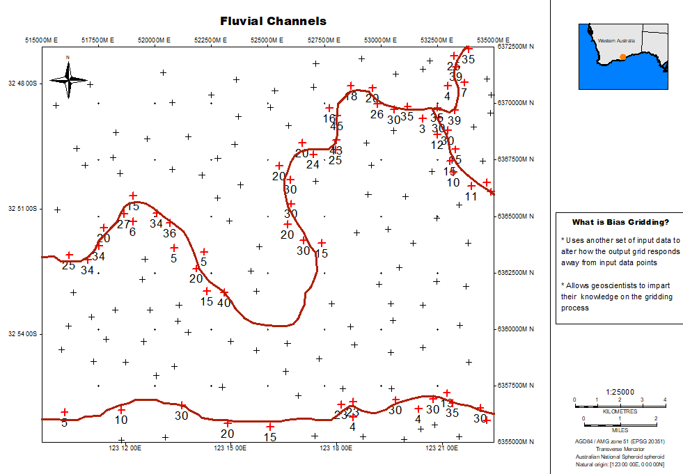
Graphic 1: Point data displaying thickness values of the channels. In red the digitised centreline of channels based on geological knowledge.
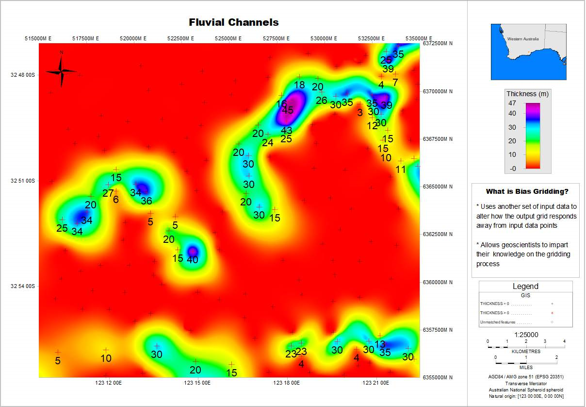
Graphic 2: Thickness grid for fluvial channels using the standard gridding operation. Notice the poor delineation of the channels.
Based on the geological knowledge of the setting mentioned above, the user could interpret the centreline of the channels and save it as a spatial dataset. This can be done in Petrosys using the Spatial Editor, a tool that allows you to edit many types of spatial datasets. This shape file can be seen in Graphic 1. Alternatively, you could use spatial data directly from a 3rd party source without having to import it. More on this in the next sections.
Once your other set of input data to guide the process is ready to be used, you will proceed to create a grid from Surface Modeling and define the parameters as with any other grid. For more information in how to create a grid, go to the Learn section in the Client Portal and have a look at the relevant workflow.
In running bias gridding, the relevant steps for this technique will come under the Methods tab:
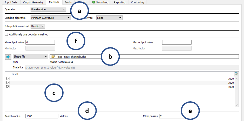
Graphic 3: ‘Methods’ tab selecting Bias-Polyline as the operation.
- Depending on the available dataset to guide the process, choose either Bias-Grid or Bias-Polyline. In this example, as we are using a spatial dataset, we select Bias-Polyline (Graphic 2).
- Select the source of the spatial data and relevant file. Notice this is the other enhancement being included in Petrosys PRO 2017, as it used to be only Petrosys Culture data that could be used to guide the process. Now you can connect and use any of the 3rd party sources that Petrosys supports without having to import the data (Graphic 4). In this example we are using a shape file.
- Select the levels to be used to create the trend.
- Define the Search Radius. This is a key parameter in the process and is used to determine the regional trend. As a rule of thumb, an initial value of search radius should be around half of the width of the channel. More info can be found in the Online Help.
- Filter passes will be the number of smoothing passes that will consider the bias distance transformation.
- Other parameters like minimum and maximum output values work in a similar way to Standard Gridding. ‘Additionally use boundary method’ provides more control over these output values.
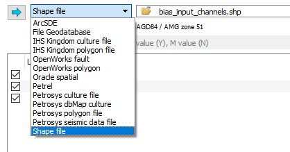
Graphic 4: Spatial data sources available to control Bias Polyline gridding. Previously only Petrosys culture data was available.
To get a good result using bias gridding, some trial and error needs to be involved. In particular when it comes to search radius and number of filter passes, different combinations should be tried before settling for a final grid.
For this example, you could see in Graphic 5 the different outputs using a different number of filter passes for a similar radius search. In all of the cases the channels are better delineated compared to the original standard gridding, thanks to the knowledge imposed on the gridding coming from the direction of the channels embedded in the spatial data.
A similar approach can be taken when there is reasonable geological knowledge that interpreters can use to guide the gridding process using Bias Gridding.
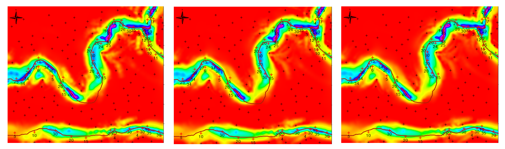
Graphic 5: Result of bias gridding with increasing number of filter passes with same search radius.
If in doubt which gridding operation you could use, contact us for some guidance and recommendations at support@petrosys.com.au or check the Learn section in the Client Portal for worfklows on how to create grids in Petrosys.