

Susanna Willan, Petrosys
Improve your mapping standards by taking advantage of the latest scientific colour gradients. We have added a number of perceptually uniform and ordered gradients to new release Petrosys PRO 2020.1, created by Fabio Crameri – a data visualisation scientist.
When assigning a colour gradient to a subsurface map, do you think about how this gradient is interpreted? Or how accessible it is for all users? Or do you apply the prettiest colours (I use this term loosely) and click publish? Research on data visualisation and scientific colour gradients has been carried out for decades and numerous authors have lamented the misuse and overuse of the rainbow colour palette, also known as the jet colour palette.
Despite this, the application of appropriate colour gradients by many geoscientists has lagged behind. I must confess that I was also late to the party. Why is this? Perhaps there has been a misconception that using the full RGB spectrum for subsurface maps will highlight the detail required for interpreting geological structures? On top of this, the rainbow colour gradient has also stubbornly embedded itself as the gradient ‘default’ for numerous software vendors. We are creatures of habit and this visual familiarisation has led to an acceptance of the ‘norm’. All I can say to that is STOP. Explore your data and explore your options, don’t accept the default just because it’s the default. Please read on…
So why is the rainbow colour palette bad for subsurface mapping?
We use visualisation methods to understand trends, patterns and structures in the underlying data. For geoscientists, colour is one of the most powerful techniques for visualising the subsurface geology in depth/time maps. Colour (along with contours) is used to quickly identify structural highs and lows, erosional and depositional features and stratigraphic thickness changes. On top of this, geoscientists use maps to analyse attributes such as porosity and net pay. Therefore, a colour palette should:
- reflect the data distribution in a uniform and ordered manner
- be accessible for those who are colour blind
- be legible in black and white print.
The rainbow gradient does none of these things. Have a look at Figure 1. Do you find yourself focussing on specific parts of the spectrum, such as the sharp contrasts at the cyan and yellow wavelengths? These are caused by a non-linear increase in brightness and result in artificial boundaries forming where none are present in reality.
![]()
Figure 1: Rainbow gradient
To illustrate this further I will compare three subsurface grids. Each grid covers the same area at a different scale. They have been displayed with the rainbow gradient and a perceptually uniform and ordered gradient. In the small-scale maps that show the regional structure of the Top Latrobe grid (Figure 2), the rainbow gradient introduces a significant amount of ‘banding’. Within these bands, our eyes are desensitised to smaller changes, especially within green and yellow wavelengths. This hides the detail that is otherwise picked up by the lapaz gradient, such as the sinuous channel that trends NW-SE before reaching the basin.
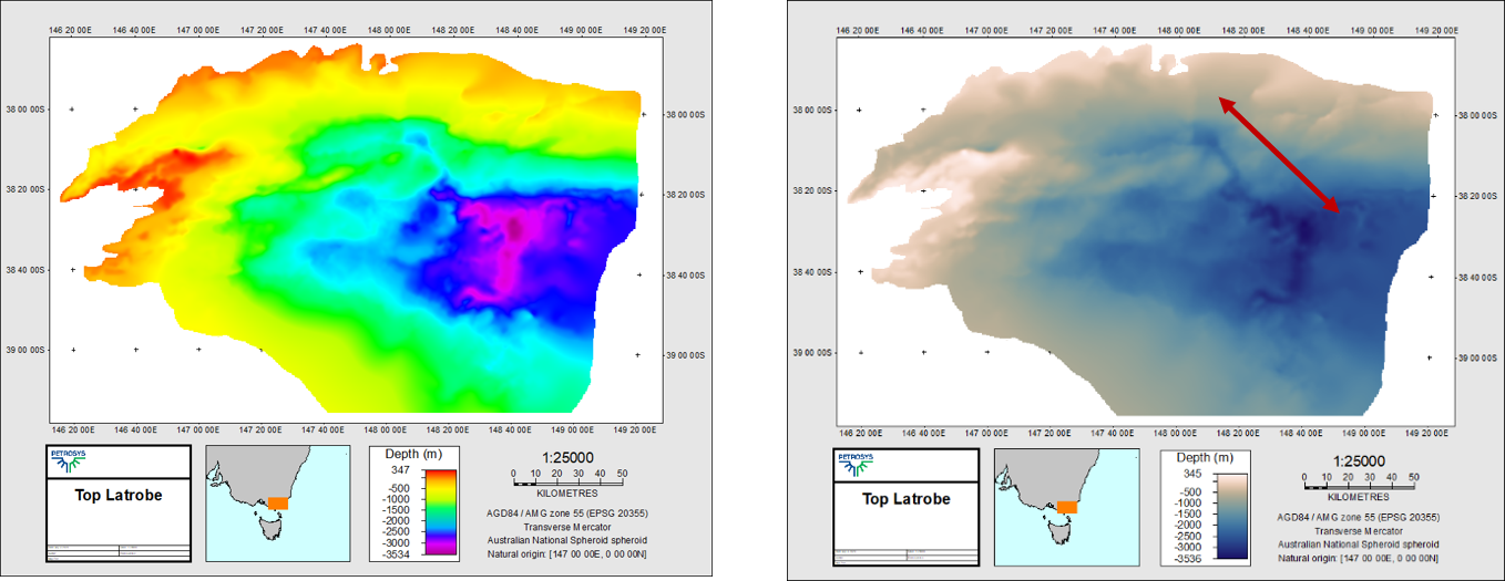
Figure 2: Top Latrobe regional grid displayed in the rainbow gradient (left) and the lapaz gradient (right).
On the medium-scale and large-scale maps, the rainbow gradient introduces two artificial boundaries to the subsurface. One has formed where the cyan and dark blue hues meet and the second where yellow and red hues meet. These unequal contrasts occur even where the contours indicate that there is little topographical change (Figure 3).
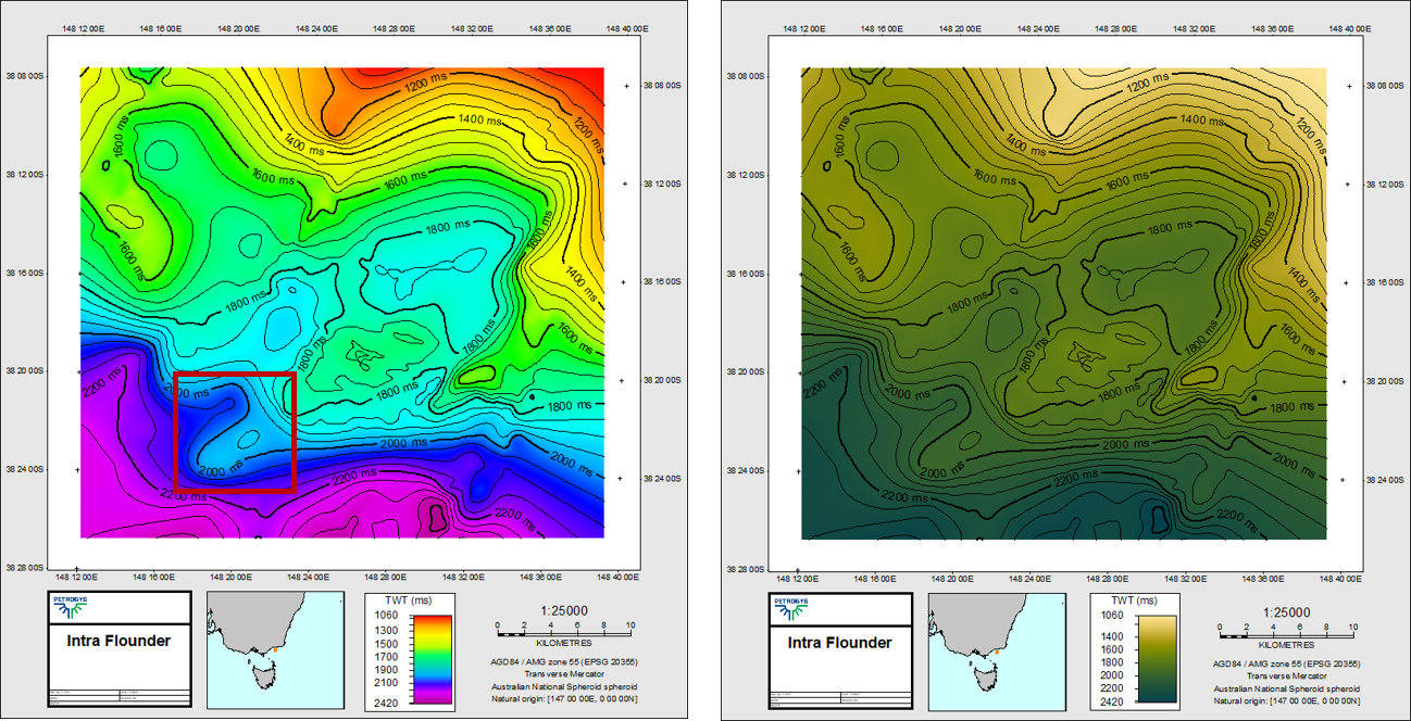
Figure 3: Intra Flounder grid displayed in the rainbow gradient (left) and the bamako gradient (right).
At prospect scale (Figure 4), this distortion makes it harder to discern the size and scale of potential structural traps. As a first pass assessment, I certainly feel more confident identifying the lowest closing contour in the right-hand map. Or rather, my eyes can interpret the subsurface geometry more accurately.
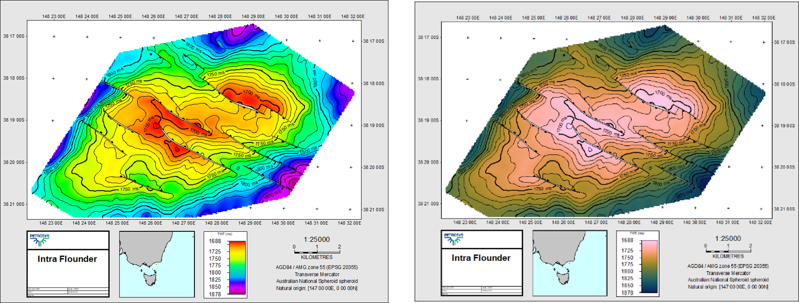
Figure 4: Intra Flounder grid displayed at prospect scale in the rainbow gradient (left) and the batlow gradient (right).
Improve your mapping standards
To avoid data misrepresentation, I would encourage you to look beyond the default colour gradients used by many software vendors. For PRO 2020, Petrosys have added a number of sequential and divergent gradients, created by Fabio Crameri. These gradients are perceptually uniform so they do not distort the underlying data and they are perceptually ordered so you can see which direction the data decreases and increases. They are suitable for people with colour vision deficiencies and they can be read in black and white prints.
So the next time you pick up a Petrosys PRO project, have a look at the new gradients added to our Gradient Selector and test these out to see how accurately they pick up erosional and structural features. Try not to settle for the default, go forth and create some beautiful scientific maps.
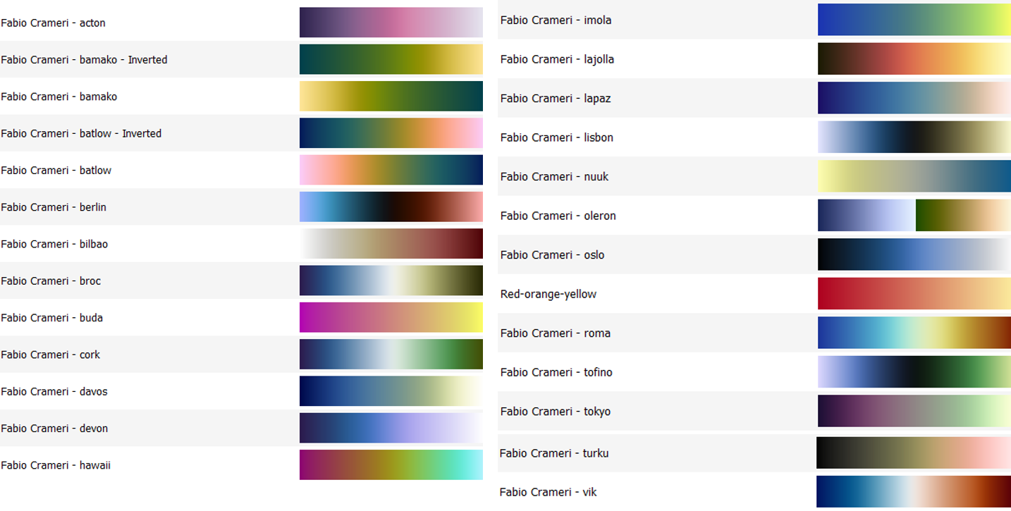
Figure 5: New gradients available in Petrosys PRO.
I want to finish with this last tip. In PRO, each new gradient is set as dynamic by default, meaning that it will automatically fit the range of the gradient to the minimum and maximum value in the input data. However, you can also fix the gradient to a user-defined minimum/maximum, or clip the range to the map extent. This is a useful function when setting a small map extent over a large regional grid. The colour gradient will reset when the map extent is moved and will display the detail required for a smaller data range (Figure 6).
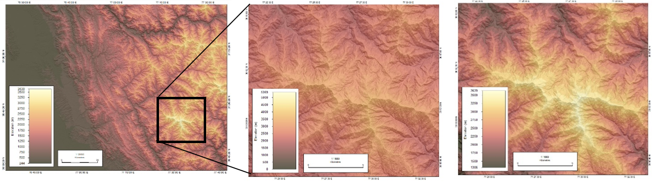
Figure 6: Difference between setting a dynamic colour range (middle) and clipping the range to the map extent (right) when displaying large regional grids. Dataset Acknowledgment: J. Takaku, T. Tadono, K. Tsutsui : Generation of High Resolution Global DSM from ALOS PRISM, The International Archives of the Photogrammetry, Remote Sensing and Spatial Information Sciences, pp.243-248, Vol. XL-4, ISPRS TC IV Symposium, Suzhou, China, 2014. Data Access granted by the Open Topography Facility (https://opentopography.org/).
Sources:
Fabio Crameri dataset http://www.fabiocrameri.ch/colourmaps.php and blog post https://blogs.egu.eu/divisions/gd/2017/08/23/the-rainbow-colour-map/
Peter Kovesi https://peterkovesi.com/projects/colourmaps/index.html
Matteo Niccoli https://mycarta.wordpress.com/category/visualization/color-visualization/
Ed Hawkins http://www.climate-lab-book.ac.uk/2014/end-of-the-rainbow/
Get in touch
If you would like to know more about Petrosys PRO contact our team of mapping gurus.