Ask Andy…Can I apply CDP geometry to 2D marine lines?

Ask Andy – Our GLOBEClaritas expert!

Q:   How can I apply CDP geometry to a 2D Marine line in Claritas?

A:  Applying a suitable 2D CDP geometry to a seismic line is a key stage of the processing sequence and in the Claritas software we have a number of options which include:

• Apply a simple 2D straight line geometry using the Griffon application and rep-defined script supplied.
• Use the MGEOM module to apply the 2D Straight line geometry.
• Use the Claritas Geometry application to apply full real world xy coordinate based geometry.

For most 2D Marine seismic lines applying a simple straight line approach for the CDP geometry is the optimal approach. It has benefits in terms of consistent fold, and regular offset distribution in the CDP domain, which makes processes like Radon demultiple easier to parameterize and more CPU efficient. There will be occasions where applying a geometry based on the real world XY coordinates is needed, however, I will cover the simple straight line approaches first.

Straight Line 2D Marine Geometry

There are two options for applying the simple straight line 2D Geometry, we can use the MGEOM module to apply as part of a Claritas job flow, or we can apply the simple 2D Geometry interactively to HDF5 datasets using a simple python script in the Griffon application. Both of these options use information from key trace headers (SOURCENUM/SHOTID/CHANNEL and COORD_SCALE) aligned with constants, defined by the user, to set the Shotpoint/Receiver/CDP interval and Near offset as well as defining the near channel and number of channels per shot record.

Which method you use will depend on a few factors, most notably how many 2D Lines you are processing and if the input dataset that you are using has all the key trace headers either set or able to be set in the Griffon application.

• If you are processing only a single line or a small number of lines then the Griffon application would be your best option.
• If you are processing a large number of lines then the option to apply geometry as part of a batch processing flow using MGEOM module may be more attractive.

Applying using the Griffon interactive application

The Claritas Griffon application allows the user to interactively apply math expressions using the Python NumPy and SciPy libraries to the seismic data’s trace header.  There is a pre-defined script to apply the simple straight line 2D Geometry to seismic data.

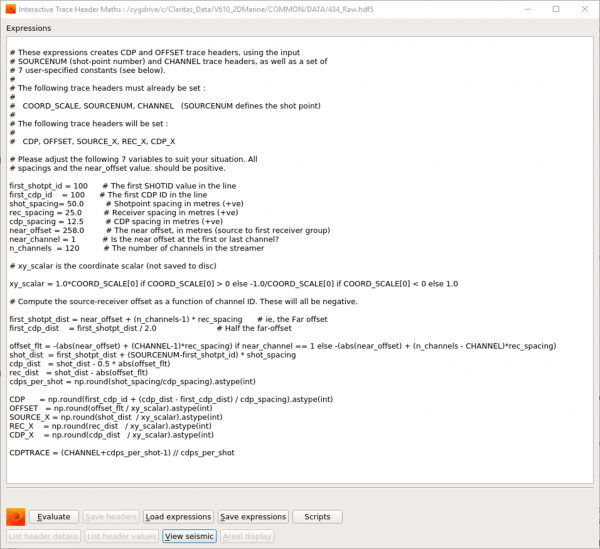
Griffon application with Simple marine geometry script.

The script sets the following trace headers in CDP/CDPTRACE/OFFSET/SOURCE_X/REC_X and CDP_X headers.

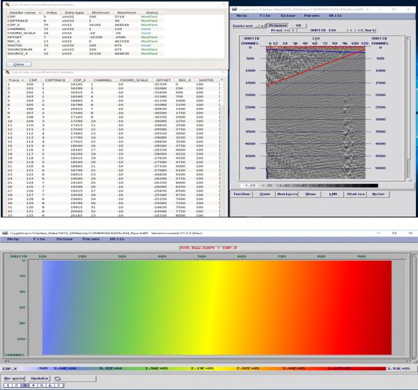
Example QC’s from Griffon – Shot gather trace headers, SV Display of shot with header overlays  and AREAL display of Offsets

Providing that the SOURCENUM/CHANNEL and COORD_SCALE headers are set by the user in the Griffon application, then this method has a number of advantges.

1. The built in QC capabilities in Griffon allow you to quickly check and confirm that the geometry has been applied correctly,
2. Minimises the use of disc space as there is no need to write out a new dataset as it updates the existing file.

Applying 2D Marine Geometry using the MGEOM module

Alternatively, if you have a large project with a significant number of lines which would make the interactive application labour intensive and not particularly efficient, you may prefer to apply the geometry as part of a Claritas batch processing job flow.  It has the same requirements as the Griffon applications script in terms of trace headers and Shotpoint/Receiver and CDP interval etc

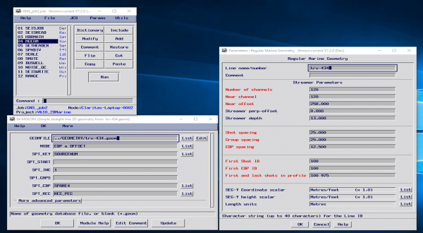
Claritas Job flow and MGEOM module and Geometry parameter form.

If required, you can set any of the required trace headers as part of the job flow using the HDRMATH/SETHEADER modules. You can add TRPRINT and RANGE modules into the job flow to provide the QC/QA  information. Otherwise, QC is performed post application viewing the results in SV/SeisView and or AREAL applications.

Geometry using Real World coordinate information from P1/90 data

In most cases when processing 2D seismic lines using straight line approximation for the Geometry is by far the best option, there are however situations where this is not the case. Being able to apply a geometry based on the real world coordinates, particularly for datasets with feathering angle issues, or high or ultra-high resolution datasets where the lateral offset of the cable from the source, will have more of an impact on the data.

For this, we will use the Claritas Geometry application and we need to reformat the UKOOA P1/90 navigation data supplied with the seismic. Ideally, this will contain both Source and Receiver position XY coordinates, but older data may only contain source positions.

Input to the Geometry application for Marine datasets can be:

• *.sht files and *.txy files: The .sht file contains source positions, and the .txy file contains the receiver positions. These can be created using the P190-to-shttxy application which can be found on the Geometry tab of the Launcher. Or they are also generated by the Claritas ADDP190 module when merging the P190 navigation data with the seismic dataset.
• *.sht and *.str files: This option is used when the P190 data doesn’t contain any receiver location information. The .sht file is created by the P190-to-shttxy application and the user creates the .str file using the XSDE spreadsheet editor. This file defines the receiver interval, Inline and Perpendicular offset, near channel, no channels, and cable depth.
• HDF5: Finally, we can also read an HDF5 seismic dataset directly into the Claritas Geometry application so if we have run a job flow where we have merged the Seismic and Navigation data using the ADDP190 module and written this out as an HDF5 dataset we can use this as input.

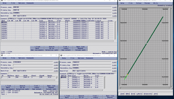
Inputs for the Geometry application (includes ,sht/,txy and .str files) and one 2D line displayed in the Geometry application before binning.

The Geometry application can be started from the Claritas Launcher by

• clicking on the Set-up button on the Geometry tab
• using the SeisCat application, selecting Geometry File type and highlighting your preferred .sht file,
• Right Mouse Button (RMB) clicking and from the drop down menu and select “Build Geometry”.

This opens the Geometry application displaying the 2D Lines SP locations in a map interface. To add the receiver information we would;

• click on the ‘Make’ button and select Create geometry database
• select the correct .str (we can use the same .str file for all lines) or .txy (unique for each line) file when the parameter form launches, this will then build a Geometry database containing both Source and Receiver position information.

We can now apply the 2D CDP Geometry, in the Geometry application there are two available methods, a linear binning scheme, and a crooked or wiggly line option. If the line is straight as in the example shown here, you can use the simpler Linear CDP Gather, the key fields are automatically parameterized based on the supplied data. You can change these if you want to, however, most are probably best left with the defaults, and changing the CDP spacing/fold and bin size along the line would be parameters that you may want to adjust.

If the line has some curvature or bends at the beginning/end or middle of the line, then you should use the Crooked line (Wiggly line CDP gather) option. When using the Crooked line option you will first need to create Hitpoints through which the lines CDP grid will pass. Typically we can use the Automatic Hitpoints option as this is robust, we then select the Wiggly Line CDP gather option and bin the data. We will be asked for the max fold of CDP’s, the CDP spacing, Bin size along the line (generally half the CDP interval), bin size perpendicular to the line large enough to allow for feather or lateral offset of the cable.

The Geometry application has some inbuilt QC capability to review fold/CDP bins etc. so you can confirm that the data has binned as you want before applying to your data. Once you are happy with the binning parameters you can merge them into the seismic trace header using either the ADDGEOM module in a processing flow or directly into an HDF5 datasets header using the ‘Save Geometry to HDF5 file headers’ option from the file drop down menu.

We have recently added a batch application utility (batch_wiggly_line) to the software in the V7.2 release which allows you to apply the Wiggly line CDP gather approach to an existing .geom  file.

To find out more about the latest GLOBEClaritas contact us and speak to the team.