
by Richard Li, Senior Software Engineer
Being a software engineer working in the Oil and Gas industry I’d say it’s quite challenging – but at the same time interesting – working in the Geomodelling domain. My previous roles had limited exposure to geoscience but through our amazing support and front-line colleagues, I see the values of providing effective toolsets for clients to model their data. Among them, generating high quality grids from various data sources is one of the key capabilities. The skilled geoscientist knows what the subsurface looks like before they generate computerized surfaces using proper tools, however, using different tools/methods will generate different resultant surfaces/grids so picking the proper/right method/algorithm, is important.
Quite often we receive clients’ queries regarding gridding algorithms /operations such as “which operation or method I should use”, “what is the difference between this operation and the other ones”, etc. We have a comprehensive collection of gridding operations to suit different scenarios: the standard one works with the least user intervention and the more advanced ones such as kriging and Kriging with Extra Drift (KED), bias gridding, localized re-gridding, etc.
So, which gridding operation should the user choose? Well, if only a part of an existing grid needs to be re-gridded, localized re-gridding could be the right choice; if a trend needs to be followed e.g. a channel/ridge/dome then bias gridding could be the best option. If the user has no specific requirements, the default i.e. the ‘standard’ operation gives the best result in most situations.
However, if a user chooses the standard gridding operation there are still further options to be considered, for example, the gridding algorithm. There are many gridding algorithms to choose from and it is at this point people ask, ‘Should I just pick the default one?’
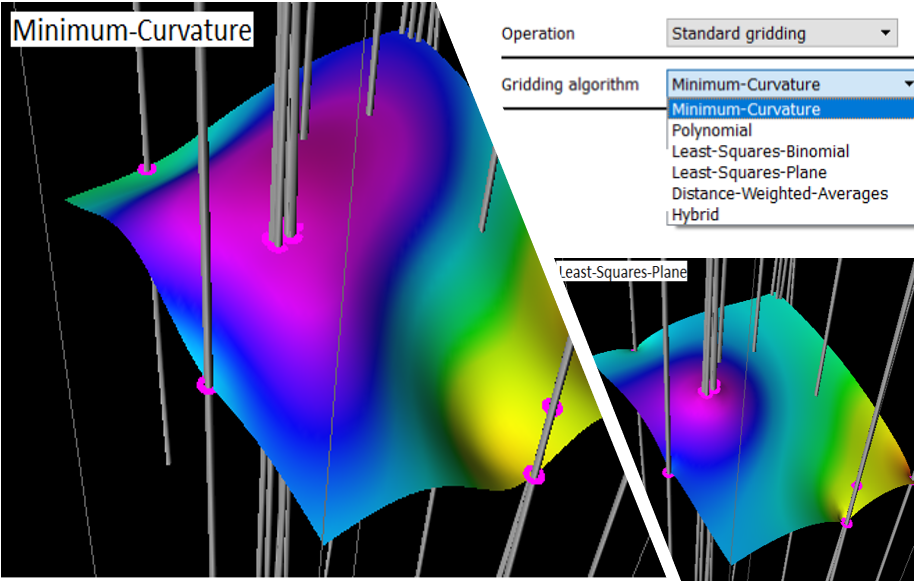
From my experience, many users do just accept the default ‘minimum-curvature’ algorithm. This is fine in most instances as minimum-curvature is the default for a very good reason and in most situations, it tends to work pretty well! However, the 5 other available algorithms (see image below) all add something different to the output surface and therefore we should always consider if they are more appropriate.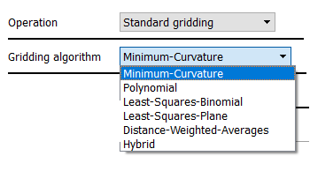
Some technical background here. Grid creation is a classical Boundary Value Problem. Over a region of interest, we want to find a discretized surface with z values that “best fit” the given known input data points. The solution of this problem is most often performed numerically by using finite difference equations approximating the derivatives at regularly spaced grid nodes, with the choice of “best fit” criteria determining which gridding algorithm to be used.
The default gridding algorithm is Minimum-Curvature which is based on minimizing the curvature of the surface. The method interpolates the data to be gridded with a surface having continuous second derivatives and minimal total squared curvature. We use an iterative method known as “relaxation” to solve the gridding problem.
A multi-grid approach is used to generate the final grid. Firstly, a course grid is generated then finer ones are generated from it until the final find grid cell size is reached. At each grid cell size the selected algorithm such as Minimum-Curvature is used to do the smoothing or “relaxation”. In detail it is first used to find a solution on a coarse grid and this solution is then interpolated as an initial estimate for successively finer grids, until the required grid geometry is achieved. At each refinement stage, the z values estimated at nodes around input points are imposed upon the grid data and a smoothing filter is applied. After each smoothing pass, the difference of the z values of the smoothed nodes near the input data point are compared with the values directly estimated from the input data and an RMS error calculated. This “forced smoothing” is repeated until some termination condition is reached before proceeding to the next finer grid cell size.
The convolution operator/matrix/pattern used during Minimum-Curvature is as follows, note that it is full a 2D one i.e. neighboring diagonal nodes are also used:
0, 0,-1, 0, 0
0,-2, 8,-2, 0
-1, 8, 0, 8,-1
0,-2, 8,-2, 0
0, 0,-1, 0, 0
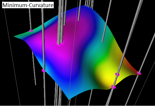
An example grid generated from well formation data using Minimum-Curvature gridding algorithm is as follows:
Other algorithms are not full 2D operators, instead 1D operators applied in both X and Y dimensions. Specifically, for “Least-Squares-Plane” it replaces a node value with the average of its four adjacent grid nodes (totally 8, 4 in X dimension and 4 in Y dimension) all with equal weights. In our standard gridding operations, the original input data points are always honored which means they will stay what they originally were during the ‘relaxation’ process. This will lead to the resultant grid has spikes at those input data points. You might visualize this grid to be a rubber sheet generally fitting the average of the data points, but “pinned” or “stretched” to also match the input data points in their immediate vicinity. Or you can think of it as “Moving Average” or simply “Average” method. The convolution operator/matrix/pattern used is as follows:
0, 0, 1, 0, 0
0, 0, 1, 0, 0
1, 1, 0, 1, 1
0, 0, 1, 0, 0
0, 0, 1, 0, 0
An example grid generated from the same well formation data using Least-Squares-Plane algorithm is as follows:
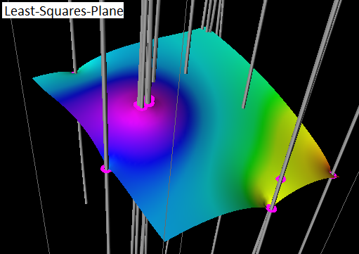
In my opinion, if the user thinks the surface should be like a rubber sheet then try Least-Squares-Plane method to see what it can produce. All of the other algorithms will work in a similar way to Least-Squares-Planes but give different results between the controlling points.
Therefore, in my view, the user needs to apply their geological knowledge and experience when it comes to picking the right methods, especially when it comes to picking different gridding operations such as Kriging, KED vs standard gridding using whatever algorithms we mentioned above. It is not possible to show the clients every detail or every line of the code to help the client to understand what each gridding algorithm/operation is doing. It is exactly the beauty of the work the support team are doing which bridges the communications between development and the end user.
It is a good question to ask, ‘to what level of detail should the application expose the algorithms to the user to configure?’. Should it be just a black box without any user intervention or should it expose as much as possible? I think there needs to be a balance and it varies from industry to industry, but what is the balance for Geomodelling application in the Oil and Gas industry and how do we achieve that balance in general? I’m happy to hear your opinions about this.
Thanks for reading to the end. If you have any queries or something I mentioned above is incorrect or anything important is missing you are more than welcome to comment or email to support@petrosys.com.au.