

Susanna Willan, Petrosys Support Geoscientist
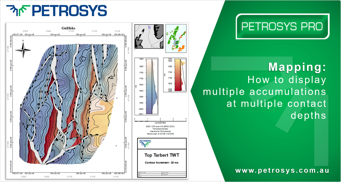
On occasion on the support desk, our Users will request help with an issue that leads to the development of a really interesting and useful workflow. In this case, our client wanted to display a top reservoir depth map that exemplifies the structure of each accumulation zone by setting transparency and colourfill independent of the lower structures.
To do this we created two workflows. The first deals with multiple accumulations that have formed at a single oil-water contact level. The second workflow discusses a more complex scenario, where multiple contact depth levels are situated across several fault blocks. In this case, a polygon boundary is generated around each accumulation and used to separate the depth grid into accumulation and non-accumulation zones.
Let’s break this down and look at it in more detail.
Workflow 1: Multiple Accumulations, One Contact Depth
Before we dive in, I want to show how quick and easy it is to display a single contact depth across a structure grid. Take the example below (Figure 1). This depth grid contains four accumulation zones that each have an oil-water contact of -1465 m.

Figure 1: Top reservoir AOI
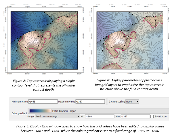
You can outline this contact depth on the original grid by setting a single contour level (Figure 2). If you want to emphasize the above-contact structures further, you can duplicate the display of the top reservoir grid. Leave the original layer displayed as described above (i.e. Figure 2). Then, for the new layer, set the minimum/maximum grid values to -1337 and -1465 (contact depth). Only the regions at, or above, the contact depth of -1465 will be displayed. Then set a fixed colour gradient of -1337 to -1860 so that the colour bar range mimics that of the original structure grid (Figure 3). Finish this off by adding transparency to the original grid.
The result will make the accumulation zones ‘pop’ whilst retaining the detail of the lower structures (Figure 4).
Workflow 2: Multiple Accumulations, Multiple Contact Levels
Ok, now onto a more complex example. Here we have a reservoir compartmentalised over several tilted fault blocks (Figure 5).

Figure 5: AOI
Each fault block contains an accumulation with a discrete contact depth – we will display these as single contact levels. Each single contour level is set up in the Contours tab of the Display Grid window (Figure 6).

Figure 6: Depth and line style defined for each single contour level.
Note: Currently the display of each contour level will be applied across the entire grid. However, for the PRO 2020.1 release, it will be possible to restrict the display of a contour level to a specified area of interest e.g. a single fault block.
The contact depths we are interested in are outlined in Figure 7. We will use the Spatial Editor and tracing technique to generate some boundary polygons.

Follow the steps outlined:
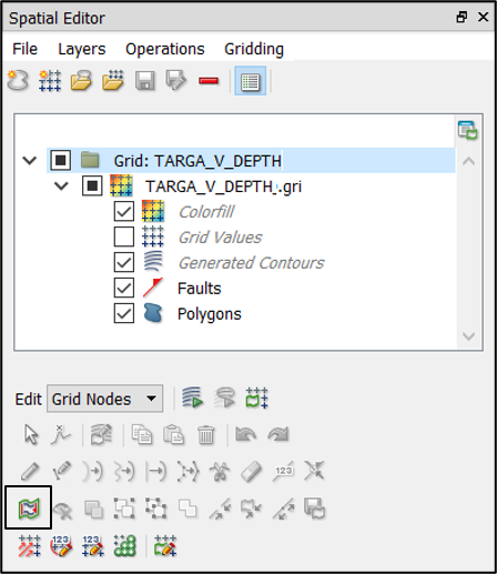
- To open the Spatial Editor, right-click on the depth grid and select Edit.
- To start digitising select the following icon (Interactively create polygon from hand-picked segments).
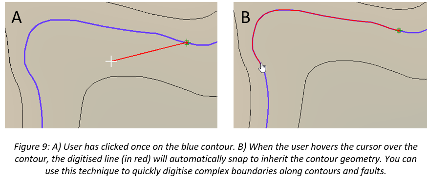
- Start digitisation by clicking on one of the single contour levels. Once that object is selected, if you hover the cursor over the same contour the digitised line will automatically snap to the line geometry (Figure 9).
Note: To undo a click, simply right click. To pan, hold down the middle mouse button
- To finish digitising, double click the mouse button.
- A window will pop up asking you to save the polygon as a file. I set the file type as Shape File and assigned the name Contact Levels.shp (Figure 10). Ensure the shape type is set as Polygon.
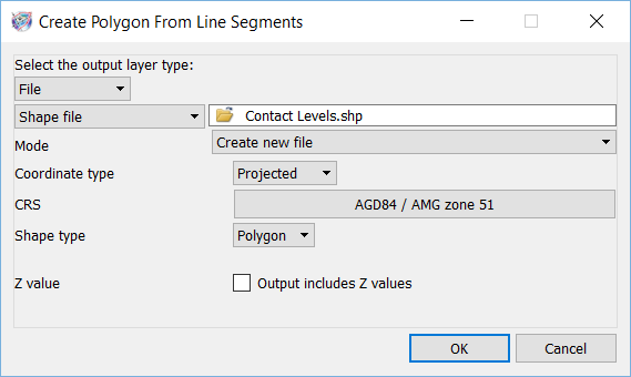
Figure 10: Creating a shape file for the polygon boundaries
- Continue digitising the remaining accumulation boundaries. Each time you double click to finish a polygon segment the window shown in Figure 6 will pop up. Set the file format to Shape file once more and make sure that the Mode is set to Update Existing File for the remaining polygons.
Once all polygons have been created you can close the Spatial Editor. To display the polygons go to Display > GIS. The polygons I created are shown in Figure 11.
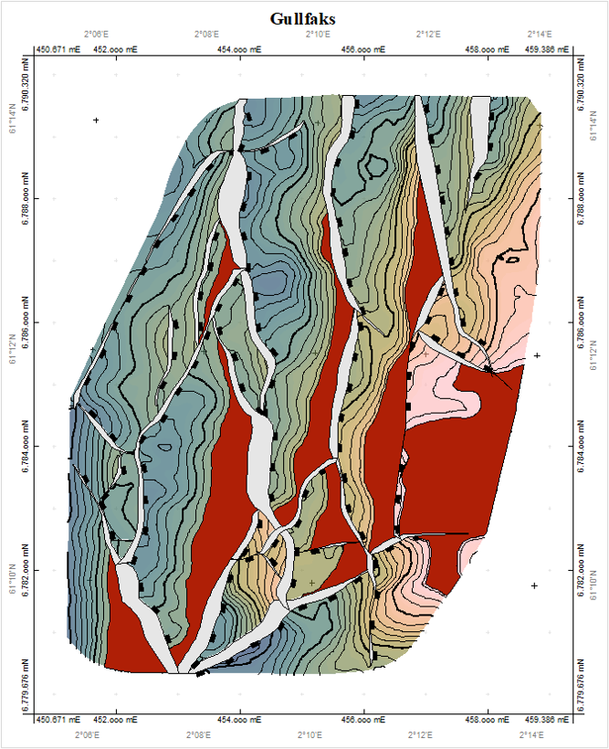
Figure 11: Accumulation boundaries digitised (shown with a red fill) where each accumulation has a different contact depth.
These polygons will now be used to extract the accumulation zones from the original structure grid. To do this:
- Go to the Petrosys PRO launcher and select Surface Modelling.
- Click Grid > Processes > Clip to Polygon (Figure 12).
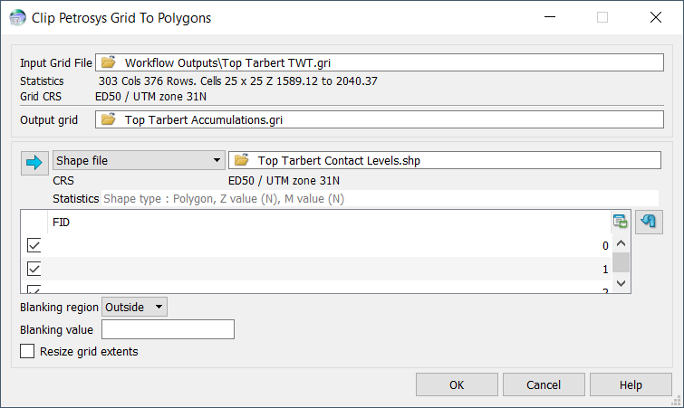
Figure 12: Clip to Polygons window
Now return to the Mapping application and display this new grid. Play around with the display options of the two grids. In Figure 13 the accumulations grid is using the same colourfill gradient and a fixed custom range so that the min/max values are the same as the original grid. The original grid has a transparency of 60% to make the accumulation zones ‘pop’.
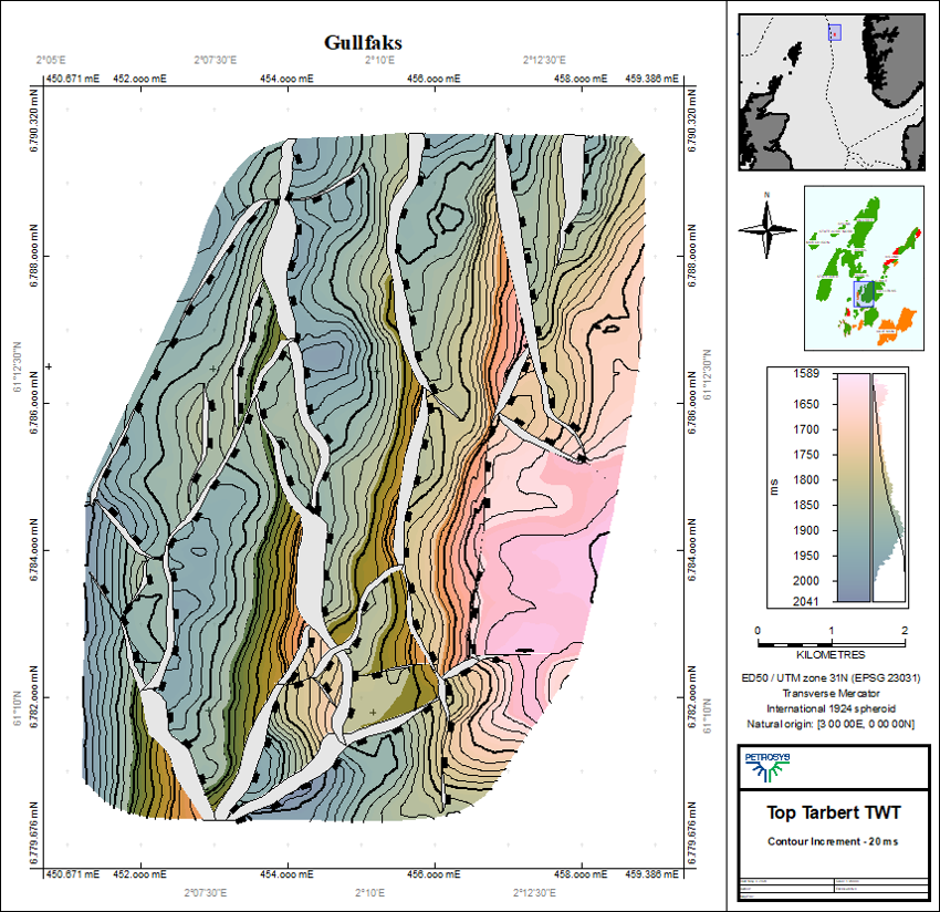
Figure 13
Alternatively, use two different colourfill gradients to further exemplify the accumulation zones from the rest of the grid (Figure 14).
Figure 14
To view more Petrosys PRO workflows log into the Petrosys Client Portal
Get in touch
If you would like to know more about Petrosys PRO contact our team of mapping gurus.