

Coal Seam Gas (CSG) (also known as Coal Bed Methane (CBM)) is the gas derived from coal seams where the coal is deep enough not to have been degraded by bacteria within the ground water and shallow enough that, when de-watered, has a low enough pressure to allow the gas to desorb from the coal and flow to surface. In CSG reservoirs, gas is stored by either lining the pores of the coal or as free gas within the natural fractures of the coal.
To determine the volume of a CSG reservoir, standard conventional volumetrics currently can’t be used in Petrosys. There are ways around this, however. The first step in conventional reservoirs is to determine the bulk rock volume (BRV). Once the bulk rock volume has been determined, one of two processes can then be followed:
- The BRV can be exported and input into a third party Monte Carlo package where other multiplying factors are applied to determine the possible range in volumetrics. This is the most common method used.
- The multiplying factors can be gridded and multiplied through the BRV grid to create a Billion Cubic Feet per Kilometre Squared (BCF/km2) grid which can then be statistically queried to determine the volume of gas in the area of interest (AOI).
At present Petrosys can’t easily back-calculate volumes from a BCF/km2 grid. The easiest way to do this is to run a statistical report from the Surface Modeling package and then use the average BCF/km2 number and multiply through by the area of the AOI to get the “Best Estimate” volume of the potential resource.
Determining bulk rock volume for CSG
The BRV of the play is determined by using several parameters:
- maturity profile
- wireline log analysis
- top and base coal grids
- well zone thickness (most Common)
Thickness
The first step is to determine the thickness of the coal. This is done by using the well logs and mud log data available as a first pass to identify coal thicknesses. This data is stored in the WDF module within Petrosys as top and base formation, and then the well data is often gridded up (where many wells are available it is a great data set to use kriging on).
Lateral Extent
The Lateral Extent of a CSG play is determined by three main factors:
- Economics of providing compression to extract the gas from the coals (too deep costs too much)
- Depth for the coals to produce gas (too shallow coals won’t produce gas)
- Regional extent of the coal seam
The lateral extent polygon and thickness grid can then be combined together to come up with a BRV within Petrosys. The probabilistic range can be used as inputs into the 3rd party Monte Carlo simulator.
CSG formulas
There are two general formulas used in CSG. The first is for exploration where little data is available on the gas composition:
OGIP (gas) = (A x H x ρ) x Gct
Where:
A = Area
H = Coal thickness
ρ = Coal density
Gct = Total gas capacity
The second involves the gas content being included to take into account any C02 or other inert gasses that will be sold at market:
OGIP (gas) = (A x H x ρ) x Gct x Gf
Where:
A = Area
H = Coal thickness
ρ = Coal density
Gct = Total gas capacity
Gf = gas fraction
Calculation methods using Petrosys
Third-party Monte Carlo method
This method is used where there is little data to back-up the model. Basically, the range of expected distributions for each input parameter are put into a Monte Carlo simulator using the simple equation above. The bulk rock volume is multiplied by the rock density to come up with a range of rock tonnage, which is then multiplied by the gas capacity (gas per weight of rock) to determine the gas in place.
Grid multiplication within Petrosys
This method can only be run if sufficient well and seismic data is available to create the required grids. The gridding method used also depends on the amount of data and the relationship of that data, ie. kriging can be a powerful method, however minimum curvature is the most common used due to lack of data in emerging basins.
Where data availability is extensive, the data can be gridded up and each grid (thickness, porosity (free gas), density and gas capacity) can then be multiplied together using grid arithmetic function within Petrosys to come up with a BCF/Km2 grid. This is becoming a common method in the unconventional industry and can also help determine sweet spots in the play. Although within Petrosys you can’t currently determine volumes from a BCF/Km2 grid, there is a way around this. Simply run grid statistics on the permit area for the BCF/Km2 grid and then multiply the average BCF by the area of the permit to come up with the average BCF of the permit. This does not work for the P90 and P10 cases.
Grids required for simple calculation:
- Thickness or bulk rock volume
- Density
- Gas capacity
- Net to gross (if used)
A typical workflow
A typical workflow for CSG would be as follows:
- Identify wells with CSG target present
- Load wells to Excel or WDF database
- Create top and base coal for target zone
- Add attributes for:
- Coal density
- Gas capacity*
- Net-to-gross
- Thickness
- Once the well data has been stored in the database each attribute can then be gridded. If there are more than 20 wells, kriging may be an option to identify trends in the data.
- If the lateral extent of the coal is known, a clipping polygon can be used to limit the extent of the grid.
- Thickness, density, gas capacity and net-to-gross grids can then be multiplied together using grid arithmetic to produce a BCF/Km2 grid (also used as the sweet spot grid to identify prospective areas).
- Display the grids in Mapping to identify prospective areas and plan well campaigns.
* Note: Gas capacity may have its own subset including ash content and moisture content volume of sorbed gas.
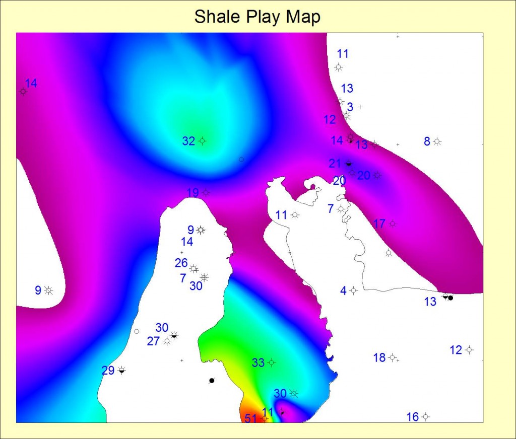
This Shale Play Map was derived by modeling the shale thickness. Prospective areas were highlighted by clipping out areas where the thickness is less than the prospective cut off (in this case 12.5m was used). The grid was also clipped where the depth was shallower than the maturity required for gas generation leaving only the prospective play area highlighted. More prospective areas are highlighted in hotter colours while less prospective areas are in cooler colours. Areas of non prospectivity are white.