
Cross validation is a technique that helps to evaluate generated grids by examining the impact that individual data points have on the grid as a whole. This method is also beneficial for assessing the input data itself. For optimal results cross validation works best with sparse datasets, such as well data.
Cross validation can be used to:
- Help identify data points that may be outliers, ie. erroneous from the rest of the dataset.
- Assist in the determination of the most suitable gridding technique or parameter setup for prediction ability.
- Provide some insight into the estimated error when drilling new locations based on a computed grid.
There are five steps involved in cross validation, which are as follows:
- The grid is computed using all available input data points.
- One data point is removed and the grid is re-computed.
- The new value in the re-computed grid is back-interpolated to the ‘missing’ point location.
- The interpolated (estimated) value for the point location is then compared with the actual known value.
- Steps 2-4 are repeated for all input data points.
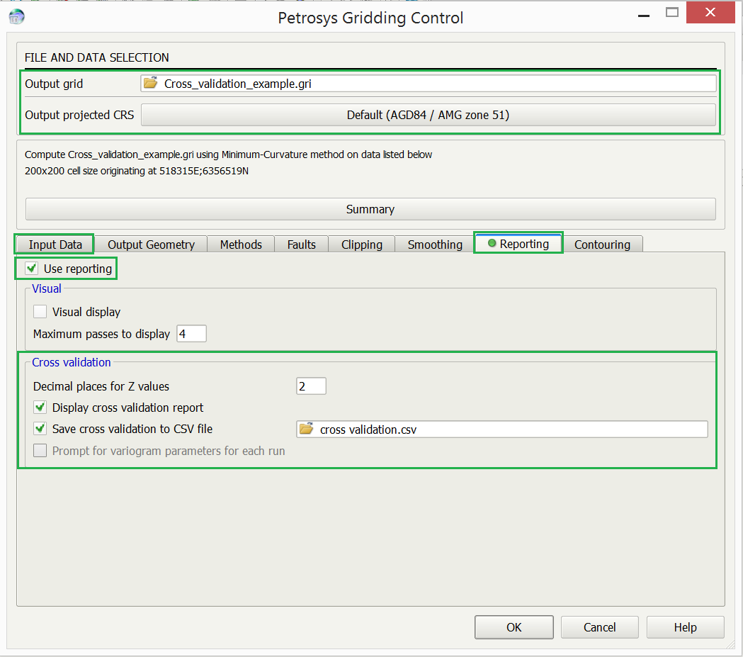
The cross validation report can be accessed during the gridding process in Surface Modeling (Grid > Create Grid) by activating the Cross validation parameters in the Reporting tab.
There are two options available – both can be selected if desired. These options are Display cross validation report and Save cross validation to CSV file.
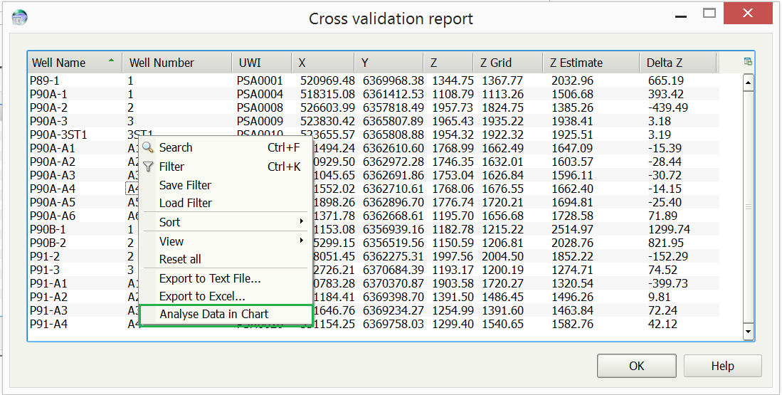
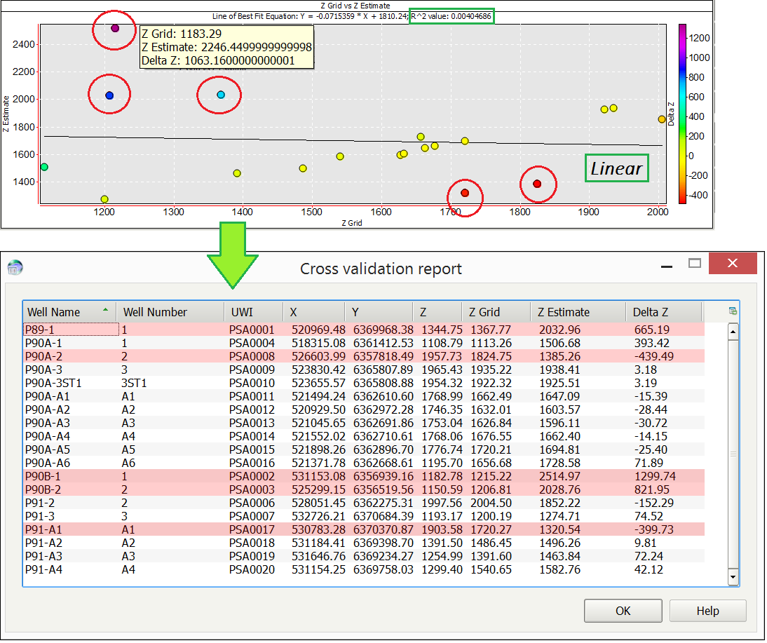
The Display cross validation report option prompts the report window to open as the gridding process is running. The report window and output .csv both consist of the input data information such as the coordinate information and the associated Z values. They also contain the Z Grid values, the Z Estimate values (the back-interpolated values) and the difference Z value known as the Delta Z. A high value for Delta Z implies that those points may be outliers/erroneous.
From the report window, cross-plotting can be accessed to view the data in chart form. This can be done using the RMB (right mouse button) and selecting the Analyse Data in Chart option.
The cross-plot can be setup using the Column Mapping options to show the correlation between the known Z values and the estimated values when the data point is removed. A good correlation indicates that the algorithm is doing a good job of predicting the data value when it is removed. The R2 value displayed on the cross-plot can be used to compare the results quantifiably. A value where R2=1 indicates that every data point available is predicted exactly by the model.
Below is an example of a dataset displayed on a cross-plot without any data points removed from the report. When any of the line of best fit options are applied the R2 value generated is very low (R2<0.1).
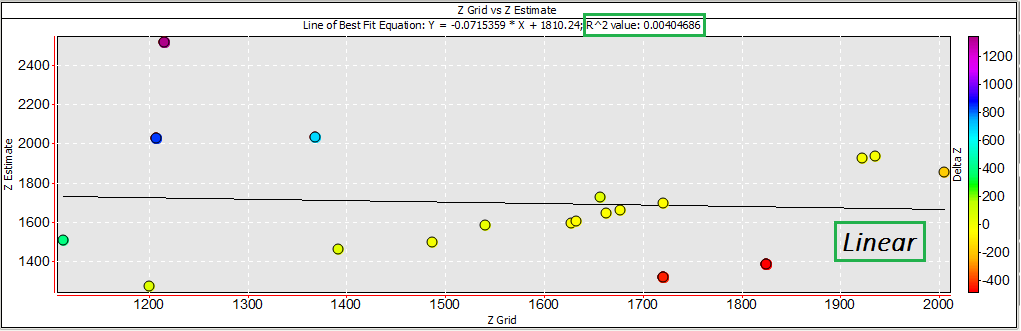
There are five points displayed on the cross-plot that appear to be outliers based on their position with relation to the Delta Z scale. Clicking on these points provides the information for the three data values displayed by each point; Grid Z, Grid Estimate and Delta Z. When clicked on, these points are also highlighted in the Cross validation report window.
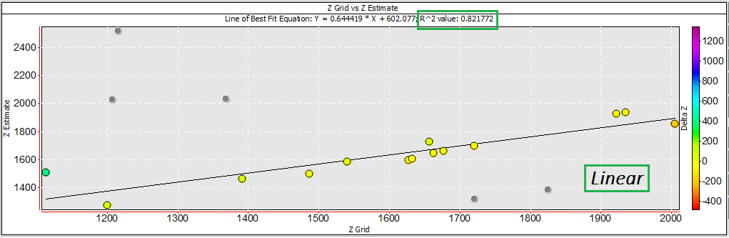
Excluding these points from the cross-plot using RMB > Exclude selected points recalculates the line of best fit and now displays a much better correlation between the datasets (R2=0.821772).
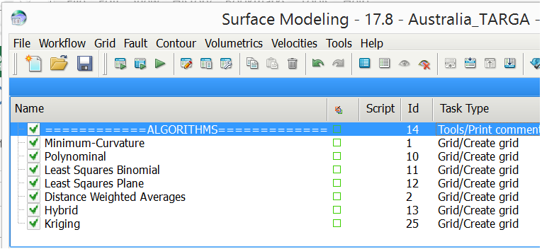
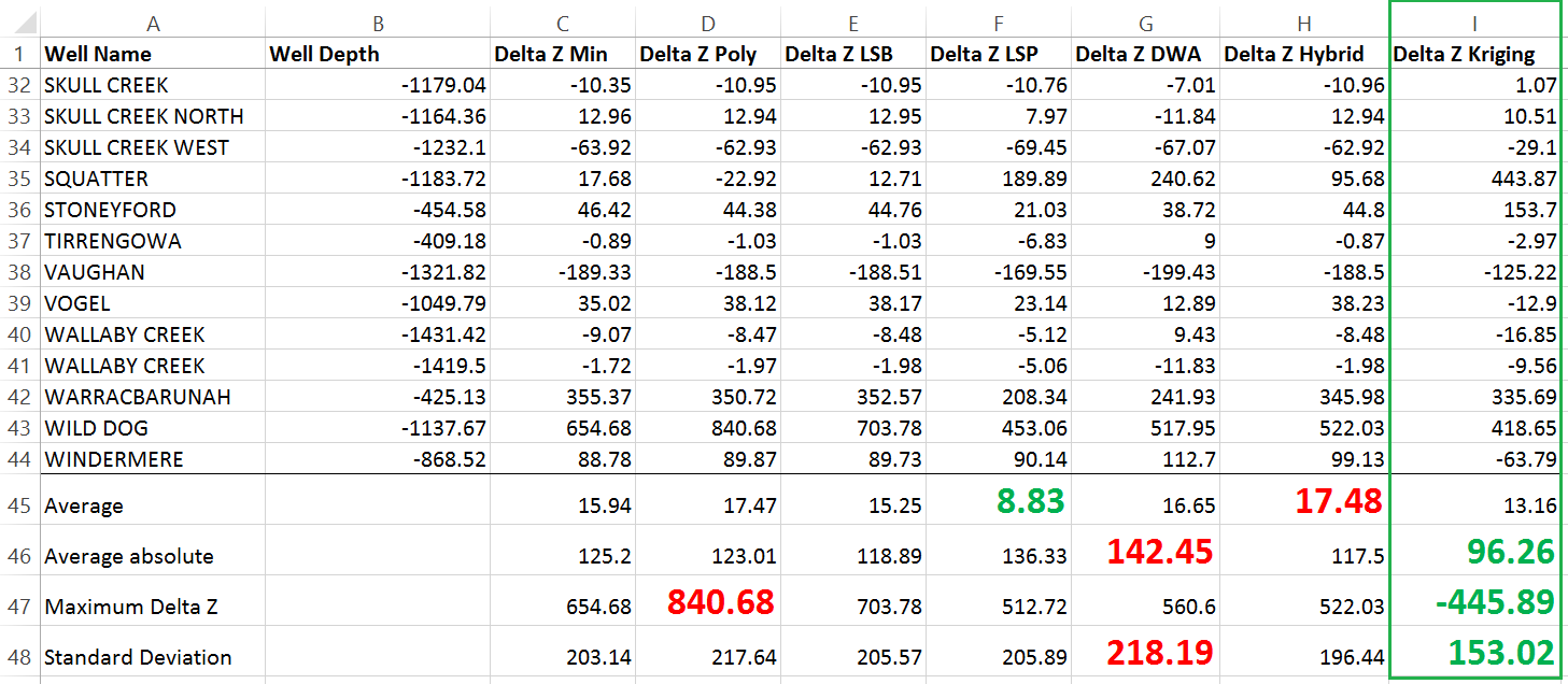
An example where the output .csv file is particularly useful is when trying to determine which gridding algorithm to use. Setting up a task file to create a grid for each of the available gridding methods and then collating the output .csv information into one file can allow for easy comparison of the Delta Z values and, therefore, make an informed decision about which gridding method is best for that particular dataset.